One of the goals of ALMAGAL is the determination of the cluster mass function (CMF) of the clusters we will detect. Irrespective on if or how CMF map into initial mass function (IMF) or not, the determination of the CMF gives important constraint for star formation models. It is also important to investigate if the CMF varies as a function of environment (galactocentric distance, vicinity to HII regions etc.) or evolutionary stage, which requires dividing the sample into subsamples.
To derive the true CMF, we have to potentially deal with four biases:
- Malmquist bias, which means that the mass detection threshold for far away sources is higher than for closer sources. Since we aim to detect 0.3 M_sun at the largest distance, this is not relevant for us.
- Flux boost or Eddington bias: the flux of sources near the detection limit can be boosted by noise, which distorts in particular the faint end of the CMF.
- Mass determination errors due to wrongly assumed temperatures. Since we often will not have a good determination of the source temperature, usually one assumes a common temperature.
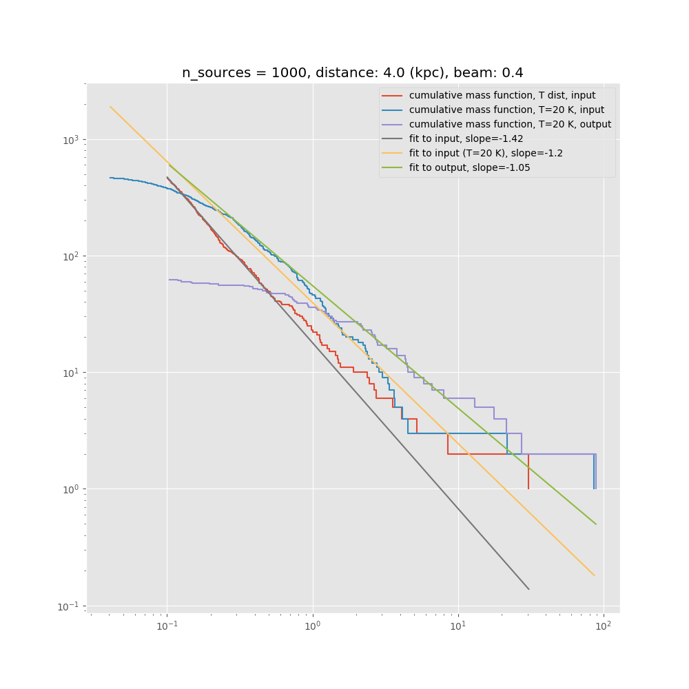
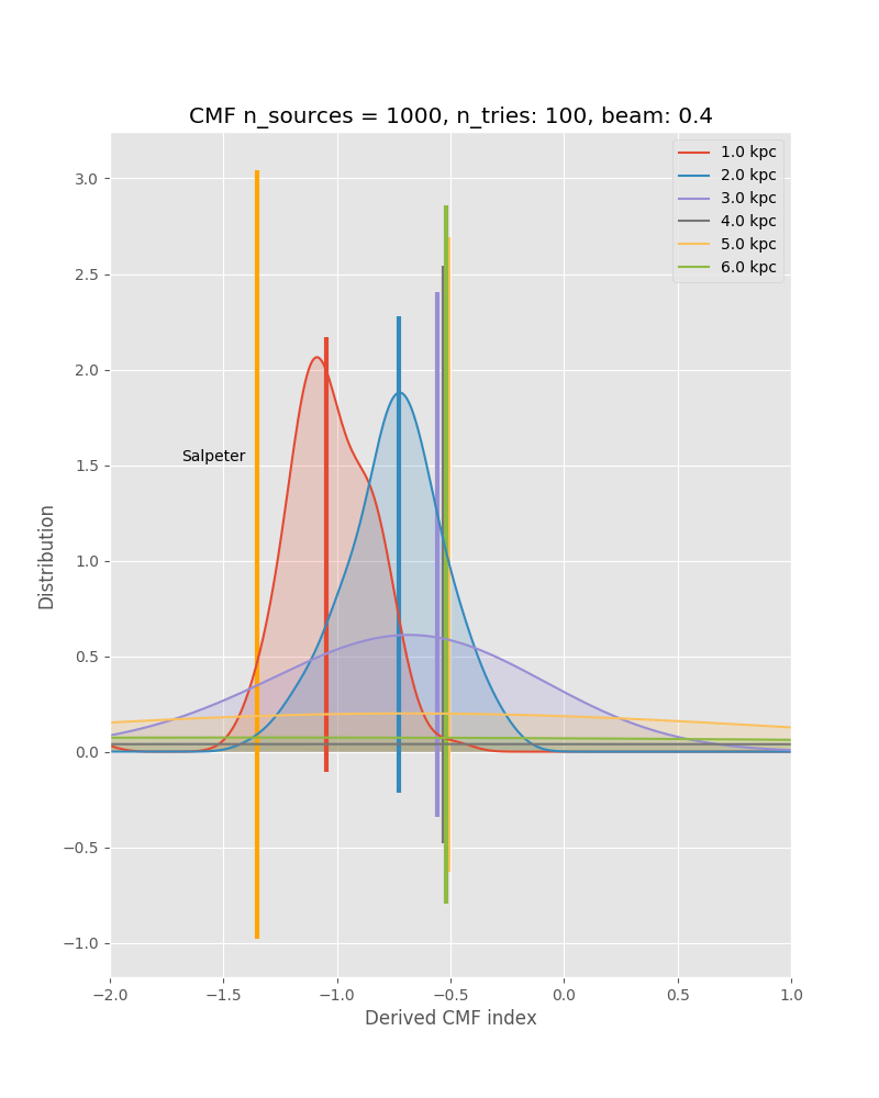
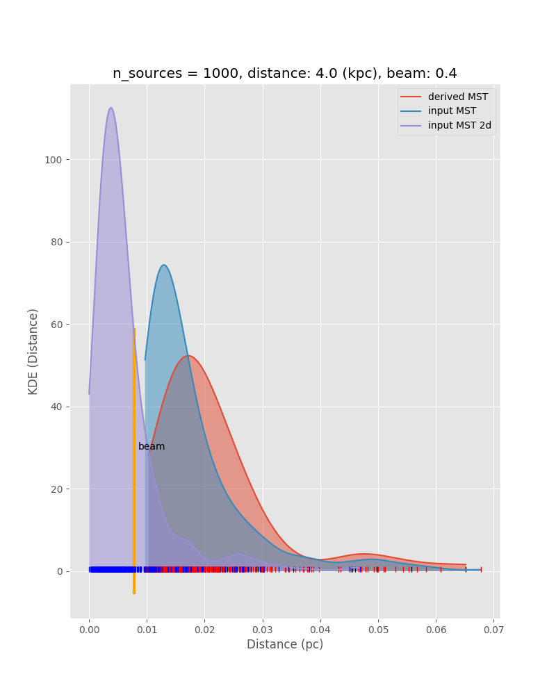
- Confusion limit: closeby low-mass sources will not be resolved, and instead of several low-mass sources enter the CMF as one higher mass source. This leads to a flattening of the CMF, which will be a function of linear resolution, i.e. the effect will get worse for larger source distances.
The confusion limit we think is the dominant effect. It could be mitigated by properly designed observations, i.e. better angular resolution for larger source distance, leading to uniform linear resolution, but it would still be there. Unfortunately, due to constraints set by the ALMA configuration schedule, this path to mitigation is not open to us.
Fortunately for us, this effect is well known and studied in the area of galaxy surveys, and since Scheuer (1957) there exists a method to correct for it: the P(D) or fluctuation analysis, which is a Bayesian method that allows to recover the original distribution from the measured one. Since 1957, this method has been developed and improved, and we particularly point out Takeuchi and Ishii (2004) who introduce the effect of clustering, which is important to us, and, as a relatively recent applications, Patanchon et al. 2009 or Glenn et al. 2010.
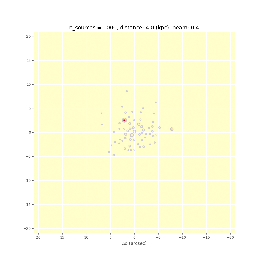
In preparation for this, we have performed Monte Carlo simulations. We model a cluster with a spatial Plummer-like distribution, but impose a minimum source distance of 2000 AU, and draw the masses out of a Salpeter IMF. In the following we show some results, such as measured CMF vs. original CMF, and measured minimum spanning tree distributions vs. the true ones from the input model. These kind of simulations together with the P(D) method will allow us to put strong constraints on the underlying true CMF. This kind of analysis depends on good statistics in all the different environmental or evolutionary bins.